The Journal of Clinical and Preventive Cardiology has moved to a new website. You are currently visiting the old
website of the journal. To access the latest content, please visit www.jcpconline.org.
Sample Size for Experimental Studies
Volume 1, Apr 2012
Padam Singh, MD, Gurgaon, India
Volume 1, April 2012
The aims and objectives of a clinical research are used in generating a “research hypothesis.” The calculation of sample size requires that we quantify the research hypothesis. The theory of statistical test of significance centers around setting a “null hypothesis.”This statistical null hypothesis is often the negation of the research hypothesis. In general the null hypothesis indicates that the effect of interest is zero or that two treatments/drugs/devices are equally effective. The “null hypothesis” is then tested against the competitive “alternative hypothesis,” indicating that the effect of interest is not zero.
While drawing inference two types of errors are encountered.
Types of Error in Hypothesis Tests
.jpg)
Type 1 error is committed when true H0 is rejected that is false claim of superiority gets accepted. The implication of Type I error in the context of a clinical trial is that the new regimen, although not effective drug, is adopted as prescribed. Thus, ineffective drug is allowed to be marketed. On the other hand, Type II error is said to be committed when false H0 is accepted that is true claim of superiority is rejected. In a trial on a new regimen, Type II error would imply that the new regimen is not approved when it is actually more effective. Thus the medical profession and the society is deprived of the benefits of this regimen.
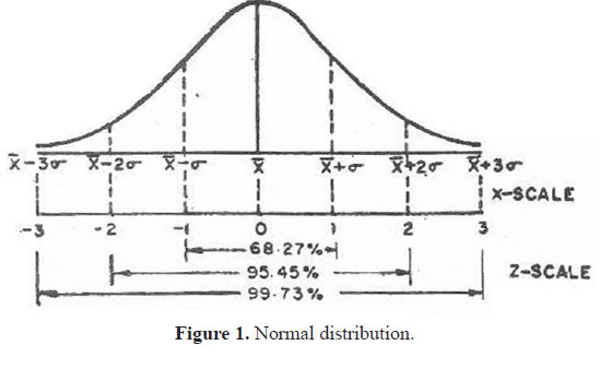
Normal distribution
Most measurements follow a pattern of the type shown in Fig. 1. The pattern has peak at the middle and rate of decline on either side has a specific pattern “bell shaped”; this is known as Gaussian or Normal distribution.
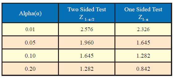
Generally, the values of standard normal variate are needed in computation of sample size for desired confidence level and power along with other assumptions. Table sowing area under standard normal curve are available to find out the values of standard normal variate corresponding to desired values of α and β. However, some of the most commonly used value of Z1-α /2 and Z1-α corresponding to different desired levels of significance are given as under:
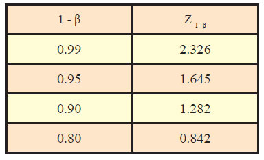
Similarly, values of standard normal variate (Z1-β) corresponding to different values of power (1-β) are as under:
Sample size for experimental studies
An experimental study is a type of evaluation that seeks to determine whether a program or intervention had the intended causal effect. Out of the various components of experimental studies, we are focusing mainly on studies/designs comparing a treatment group and a control group.
Clinicians are not at ease with formulae and computations. Therefore tables have been prepared for use by them,which could serve as ready reckoners in determining the sample size for a given situation.
In studies, the outcome variable for evaluation could be binary, such as “cure rate” or “survival rate,” efficacy, etc. Also there are studies aimed at evaluating the changes in the parameters which are of continuous nature such as BP measurements, HbA1C values, etc. The computation of sample size is discussed separately for both types of outcomes.
.jpg)
Binary outcome
In most experimental studies, a new drug is compared for its efficacy with the standard drug as control. The sample size in this situation is determined based on the following information:
Normal distribution
Most measurements follow a pattern of the type shown in Fig. 1. The pattern has peak at the middle and rate of decline on either side has a specific pattern “bell shaped”; this is known as Gaussian or Normal distribution.
Generally, the values of standard normal variate are needed in computation of sample size for desired confidence level and power along with other assumptions. Table sowing area under standard normal curve are available to find out the values of standard normal variate corresponding to desired values of α and β. However, some of the most commonly used value of Z1-α /2 and Z1-α corresponding to different desired levels of significance are given as under:
Similarly, values of standard normal variate (Z1-β) corresponding to different values of power (1-β) are as under:
Sample size for experimental studies
An experimental study is a type of evaluation that seeks to determine whether a program or intervention had the intended causal effect. Out of the various components of experimental studies, we are focusing mainly on studies/designs comparing a treatment group and a control group.
Clinicians are not at ease with formulae and computations. Therefore tables have been prepared for use by them,which could serve as ready reckoners in determining the sample size for a given situation.
In studies, the outcome variable for evaluation could be binary, such as “cure rate” or “survival rate,” efficacy, etc. Also there are studies aimed at evaluating the changes in the parameters which are of continuous nature such as BP measurements, HbA1C values, etc. The computation of sample size is discussed separately for both types of outcomes.
Binary outcome
In most experimental studies, a new drug is compared for its efficacy with the standard drug as control. The sample size in this situation is determined based on the following information:
- Approximate value of efficacy/cure rate for standard treatment (e.g., 60%) = P1
- Approximate value of efficacy/cure rate for new drug (e.g., 80%) = P2
- Effect size (i.e., difference in efficacy of control and experimental group, e.g., 20%) = (P2-P1)
- Level of significance (usually 5%)
- How high should the probability of obtaining
- significant result be (“power,” e.g., 90%)?
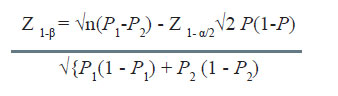
The formula used in the situation is as under:
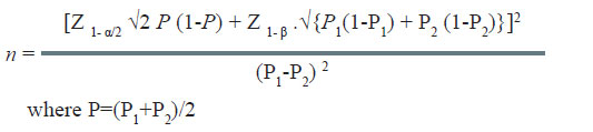
In the above example, the efficacy/cure rate on standard treatment is 60%. The new treatment would be considered superior if it offers at least 20% more over the standard treatment. It is desired to estimate the minimum number of patients required in each group in this study. The computation of sample size is as under:
In the above example, the efficacy/cure rate on standard treatment is 60%. The new treatment would be considered superior if it offers at least 20% more over the standard treatment. It is desired to estimate the minimum number of patients required in each group in this study. The computation of sample size is as under:
Here, P1 = 0.6, P2= 0.8
P = (0.6 + 0.8)/2=0.7
α = 0.10, β = 0.20
Therefore;
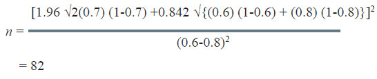
Therefore;
The sample size to study the above claim with 95% confidence level and 80% power will be 82.
In this very example, other thing remaining the same, if the power of the test is changed from 80% to 90%, the sample size increases from 82 to 105 as could be seen from table below:
.jpg)
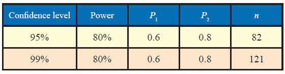
Similarly, if confidence level is increased from 95% to 99%, the sample size increases from 82 to 121.
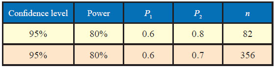
Further, if the effect size (P2-P1) is 10% as against 20%, then also the sample size increases from 82 to 356 .
In view of above, the sample size calculations should be based on our best guesses of the situation and realistic assumptions because of the following facts:
- Sample size will be higher for higher power of detecting the difference as significant
- Sample size will be higher for higher confidence levels
- Sample size will be higher for detecting an effect size which is of smaller magnitude
Many a times, the investigator uses a lower sample size than desired. In that case, the implications of the reduction in sample size could be examined statistically. Also, the estimated effect size could be different than assumed, the implication of which could also be analyzed using statistical principles.
In this case besides confidence level and power, theother information required is as under:
Example:In this case besides confidence level and power, theother information required is as under:
a. mean of the outcome variable in group 1 = M1
b. mean of the outcome variable in group 2 = M2
c. SD of the outcome variable in group 1 = σ1
d. SD of the outcome variable in group 2 = σ2
The formula used in calculation of sample size is given below:
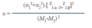
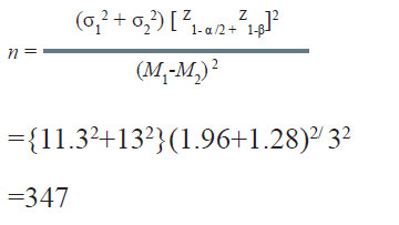
A nutritionist wishes to study the effect of lowering sodium in diet on systolic blood pressure (SBP). During a pilot study, it was observed that the standard deviation of SBP in community with a low sodium diet was11.3 mmHg while that with high sodium diet it was 13.0 mmHg. If α = 0.05 and β = 0.10, how many persons from each community should be studied if one wants to detect 3.0 mmHg difference in SBP in the two communities as significant?
Solution:
Solution:
Therefore, a minimum of 347 persons from each community would be required to be included in the study.
Equivalence of two interventions
When the standard therapy is invasive, expensive, or toxic and the experimental therapy is conservative, one may be interested in showing that the experimental therapy is equivalent in efficacy of standard therapy, rather than necessarily superior.
In this situation, the null hypothesis may specify that the difference in success rate of the control therapy (Pc) and standard therapy (Ps) by up to d amount will be considered equivalent.
The sample size for equivalence studies is calculated using the following formula:
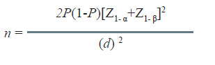
Here, Pc = Ps = P
Equivalence of two interventions
When the standard therapy is invasive, expensive, or toxic and the experimental therapy is conservative, one may be interested in showing that the experimental therapy is equivalent in efficacy of standard therapy, rather than necessarily superior.
In this situation, the null hypothesis may specify that the difference in success rate of the control therapy (Pc) and standard therapy (Ps) by up to d amount will be considered equivalent.
The sample size for equivalence studies is calculated using the following formula:
Here, Pc = Ps = P
Example:
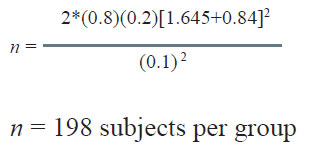
If the underlying 5-year survival rate in two groups is 80% and the threshold for equivalence is 10%, the sample size required for establishing equivalence with 80% power and 95% confidence level is as under:
Computation of power
The steps involved are as under:
Illustration 1
Computation of power
Many times it is desirable to compute the power of the study for given sample size and other assumptions. The formula used in this case is given by
The steps involved are as under:
- Compute Z1- β using the above formula for given n, P1, P2, and α.
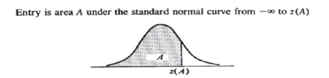
- Then making use of the table of normal distribution, find the cumulative probability corresponding to the calculated value of Z1- β.
Illustration 1
In the example considered earlier, if the resulting sample size is 64 as against 82 planned, the power is computed as under:
Illustration 2
The value of Z1- β works out as 0.50.
The area of the normal curve upto 0.50 is 0.6915.
Thus the power of the study reduces to 69.15% as against 80% planned.
Illustration 2
In the example considered earlier, if the difference resulting as significant is 10% as against 20% assumed, in that situation the power is computed as under:
Adjustment for Varying Sample Size
The value of Z1- β works out as -0.62.
Area of the normal curve upto -0.62 is 0.2716. Thus the power reduces to 27.16%.
Adjustment for Varying Sample Size
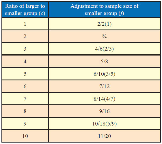
Many a times, it may not be possible or even desirable to have same sample size for each group. It may be of interest to know as to what difference would it make on the inference if the sample size varies in two groups as well as what way it could be adjusted for desired results. Table 1 gives appropriate adjustment factors for the number of sample in the experimental group according to the differing ratio of sample in the experimental versus control groups.
If n is the estimated sample size for equal-size groups and the size of the larger group is desired to be c times that of the smaller group, factor (f) is applied to the smaller group which equals (c + 1)/(2c), in this case, the sample size of the smaller group is “fn” and that of the larger group as “cfn.”
Adjustments for loss to follow-up
Adjustments for loss to follow-up
It is generally the case that some of the subjects originally recruited in the study might be lost to followup or withdraw. Thus, the calculated sample size should be increased to allow for possible nonresponse or loss to follow-up.
For example, if x= 20% the multiplying factor equals 100/(100 - 20) = 1.25.
Adjustment for confounding
Adjustment for clustered designs
Design effect (Deff) = 1+ (n’-1) × ICC
where ICC = intraclass correlation coefficient
n’ = average cluster size
Adjustment factor for x% loss=100/(100 - x)
For example, if x= 20% the multiplying factor equals 100/(100 - 20) = 1.25.
Adjustment for confounding
If there is a likelihood of a confounding variable, to adjust for the effect, the sample size is required to be increased by 10% (1). For several confounding variables
that are jointly independent, as a rough guide one could add the extra sample size requirements for each variable separately.
Adjustment for clustered designs
In cluster randomized trials, in which randomization is applied to clusters of people rather that individuals, the sample size is require to be adjusted for clustering effect. The amount by which the sample size needs to be multiplied is known as design effect (Deff), which depends on the intraclass correlation coefficient (ICC).
Design effect (Deff) = 1+ (n’-1) × ICC
where ICC = intraclass correlation coefficient
n’ = average cluster size
For more details about sample size calculation for cluster randomized trials, readers are advised to refer to Donner and Klar (2).
References
Further Reading
References
- Smith PG, Day NE. The design of case-controlled studies: the influence of confounding and interaction effects. Int J Epidemiol. 1984; 13:356–65.
- Donner A, Klar N. Design and Analysis of Cluster Randomization Trials in Health Research. Arnold: London; 2000.
Further Reading
- Kirkwood BR, Sterne JAC. Medical Statistics, 2nd edition. Oxford: Blackwell Science Ltd; 2003.
- Pandey RM. Sample Size Calculation. Lecture Notes, 2010.